Plot and Inspect Signals in Trace, Periodogram, and Histogram

Usage

diagnose_signal(
  s1,
  s2 = NULL,
  sc = NULL,
  srate,
  name = "",
  try_compress = TRUE,
  max_freq = 300,
  window = ceiling(srate * 2),
  noverlap = window/2,
  std = 3,
  cex = 1.5,
  lwd = 0.5,
  flim = NULL,
  nclass = 100,
  main = "Channel Inspection",
  col = c("black", "red"),
  which = NULL,
  start_time = 0,
  boundary = NULL,
  mar = c(5.2, 5.1, 4.1, 2.1),
  ...
)

Arguments

s1: Signal for inspection
s2: Signal to compare, default NULL
sc: compressed signal to speedup the trace plot, if not provided, then either the original s1 is used, or a compressed version will be used. See parameter try_compress.
srate: Sample rate of s1, note that s2 and s1 must have the same sample rate
name: Analysis name, for e.g. "CAR", "Notch", etc.
try_compress: If length of s1 is too large, it might take long to draw trace plot, my solution is to down-sample s1 first (like what Matlab does), and then plot the compressed signal. Some information will be lost during this process, however, the trade-off is the speed. try_compress=FALSE indicates that you don't want to compress signals under any situation (this might be slow).
max_freq: Max frequency to plot, should be no larger than half of the sampling rate.
window: Window length to draw the Periodogram
noverlap: Number of data points that each adjacent windows overlap
std: Error bar (red line) be drawn at standard deviations, by default is 3, meaning the error bars represent 3 standard deviations.
cex, lwd, mar, ...: passed to plot.default
flim: log10 of frequency range to plot
nclass: Number of classes for histogram
main: Plot title
col: Color for two signals, length of 2.
which: Which sub-plot to plot
start_time: When does signal starts
boundary: Boundary for signal plot, default is 1 standard deviation

Examples

library(stats)
time <- seq(0, 100, by = 1/200)
s2 <- sin(2 * pi * 60 * time) + rnorm(length(time))
diagnose_signal(s2, srate = 200)

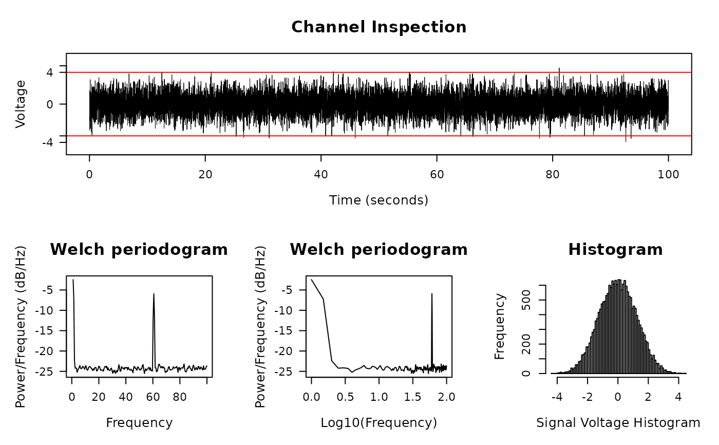#> $ylim
#> [1] 4.431596
#> 
#> $boundary
#> [1] 3.674513
#> 

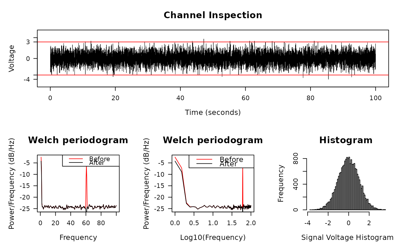
# Apply notch filter
s1 = notch_filter(s2, 200, 58,62)
diagnose_signal(s1, s2, srate = 200)

#> $ylim
#> [1] 3.755492
#> 
#> $boundary
#> [1] 2.98199
#>